1.7 Rational Functions and End Behavior

1.7 Rational Functions and End Behavior

Let’s give our lovely friend—the polynomial function—a break and move on to the other major players in this unit: rational functions! We’ll first define what they are; chances are, you already know what they are but do not realize they’re called… well, rational functions. Then, we’ll define their end behaviors similar to the previous section. Woo-hoo! 🥂

🪄 New Character Unlocked: Rational Functions

Head’s up: Technically, our friend Poly Nomials is not retiring. Their role is being expanded with the help of rational functions! 🎩

You might wonder: How come?

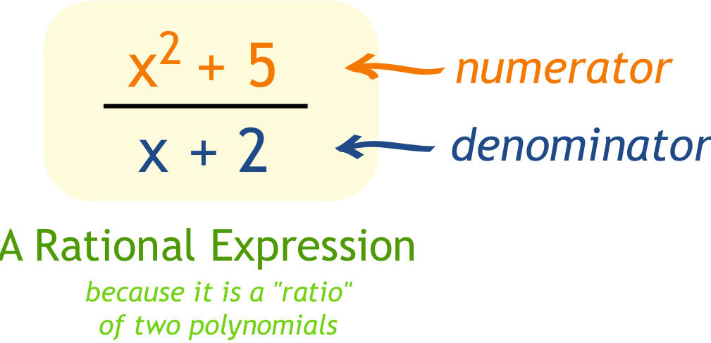
Well, a rational function can be expressed as the quotient of two polynomial functions. In other words, it is a ratio of two polynomials. The numerator and denominator of the rational function are themselves polynomial expressions. The degree of the polynomial in the numerator and the degree of the polynomial in the denominator determine the behavior of the rational function.

The rational function measures the relative size of the polynomial function in the numerator with respect to the polynomial function in the denominator for each value in its domain. This ratio of polynomial functions is crucial in understanding the behavior of the rational function.

Image Courtesy of Math is Fun

For instance, if the degree of the polynomial in the numerator is less than the degree of the polynomial in the denominator, then the rational function approaches zero as the input values get large. Conversely, if the degree of the polynomial in the numerator is greater than the degree of the polynomial in the denominator, then the rational function approaches infinity or negative infinity as the input values get large. 😳

🔚 End Behaviors

The behavior of a rational function at the ends of its domain can be determined by looking at the degree of the polynomial in the numerator and the denominator. 🔥

The polynomial with the higher degree will have the greatest influence on the overall behavior of the rational function. This is because, as input values become larger, the leading term of the polynomial with the higher degree will dominate the leading term of the other polynomial, and consequently, it will also dominate the behavior of the rational function.

To better understand the end behavior of a rational function, we can examine the quotient of the leading terms of the polynomial in the numerator and the polynomial in the denominator. 🔎

(1) Numerator Polynomial Dominates

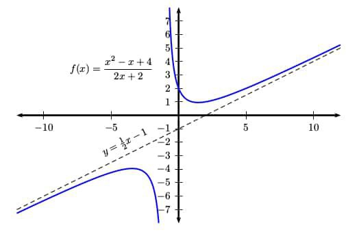
If the leading term of the polynomial in the numerator is larger than the leading term of the polynomial in the denominator, then the quotient of the leading terms will be a non-constant polynomial. In this case, the original rational function will have the same end behavior as this polynomial. 🔝

If the quotient of the leading terms is a linear polynomial, then the rational function will have a slant asymptote that is parallel to the graph of the line. This is because the linear polynomial has a constant slope, which means that the graph of the rational function will approach the slant asymptote at a constant rate.

Image Courtesy of Quora

(2) Neither Polynomial Dominates

If neither polynomial dominates the other for input values of large magnitude, then we need to look at the quotient of their leading terms. This quotient will be a constant, and this constant will indicate the location of a horizontal asymptote for the graph of the original rational function. The horizontal asymptote will be at the same level as this constant. 😐

(3) Denominator Polynomial Dominates

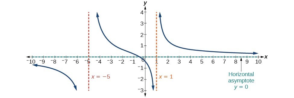
If the polynomial in the denominator dominates the polynomial in the numerator for input values of large magnitude, then the quotient of the leading terms will be a rational function. ⬇️

In this case, the numerator will be a constant, while the denominator will be a non-constant polynomial. The graph of the original rational function will have a horizontal asymptote at y = 0. This is because, as input values become larger, the denominator will dominate the numerator, causing the overall value of the rational function to approach zero.

Image Courtesy of Quora

🛑 Limits

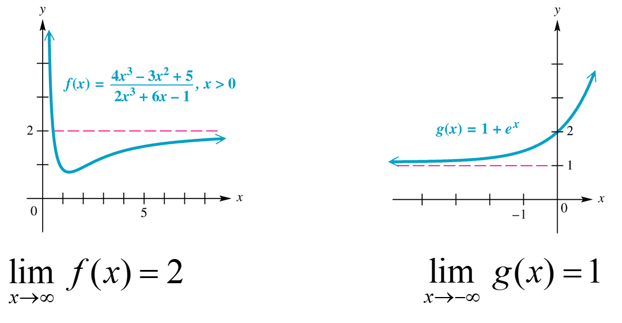
When a rational function r has a horizontal asymptote at y = b, this means that as the input values of the function increase or decrease without bound, the output values of the function will approach the constant value of b. Moreover, the function will stay arbitrarily close to the value of b as the input values continue to increase or decrease. We use the limit notation to express this behavior mathematically. 😓

Specifically, we write:

• lim r(x) = b as x approaches positive or negative infinity,

which indicates that the limit of the function approaches the constant value of b as the input values increase or decrease without bound.

This horizontal asymptote behavior can be observed in the graph of the function, where the curve approaches a straight line at the value of y = b but never touches or crosses that line.

Image Courtesy of W3 Schools